1. 概要: β多様性とは
2. R vegdist() 関数による β 多様性の計算
   • dune データセット
   • 計算
   • 結果の表示と保存
3. cmdscale() および ggplot() による図の作成

概要: β多様性とは

β多様性は、2 つのサンプルや地点間での生物多様性を示す指標である。2 つのサンプルがどれくらい似ているか (または似ていないか) が数値として与えられる。

他にも α多様性および γ多様性があるので、基礎的な内容については以下のサイト内検索から関連ページを参照のこと。

β多様性を表す指数としては、Bray-Curtis 距離 や Jaccard 距離 などがある。このページでは、R の vegdist() 関数を用いてこれらの距離を算出する方法をまとめる。

R vegdist() 関数による β 多様性の計算

dune データセット

R によるα多様性の計算 と同じく、vegan という パッケージ と、このパッケージに含まれている dune という 組み込みデータセット を用いる (表は dune の一部)。20 行 30 列のデータである。

library(vegan)
data(dune)

行は場所であるが、単に 1 - 20 の番号が割り振ってある。列の Achimill, Agrostol などは種名の略称で、

make.cepnames

を実行すると、この略称を作った関数をみることができる。

計算

vegdist() 関数でβ多様性を計算する。

dis.bc <- vegdist(dune, method = "bray")

とすると、20 個のデータの総当たりで Bray index が表示される。

つまり、input は abundance のみを含むデータフレームである。

method はさまざまな方法が指定可能で、Documentation には "manhattan", "euclidean", "canberra", "bray", "kulczynski", "jaccard", "gower", "altGower", "morisita", "horn", "mountford", "raup" , "binomial", "chao", "cao" or "mahalanobis" が載っている。調べたものを表にした。

距離なので、どれも「2 つの記録がどれくらい異なっているか」という指標である。

gower	Gower 距離、Gower’s Distance (4)。データに logical, categorical, numerica, text が混在していても計算できる。0 から 1 の間の値をとり、0 が完全に同一、1 が最大限に異なる。
altGower	Manual より引用。 There are two versions of Gower distance ("gower", "altGower") which differ in scaling: "gower" divides all distances by the number of observations (rows) and scales each column to unit range, but "altGower" omits double-zeros and divides by the number of pairs with at least one above-zero value, and does not scale columns (Anderson et al. 2006). You can use decostand to add range standardization to "altGower" (see Examples). Gower (1971) suggested omitting double zeros for presences, but it is often taken as the general feature of the Gower distances. See Examples for implementing the Anderson et al. (2006) variant of the Gower index.
bray
manhattan	量的データ、つまり比率尺度または間隔尺度のデータに適用される (図は public domain)。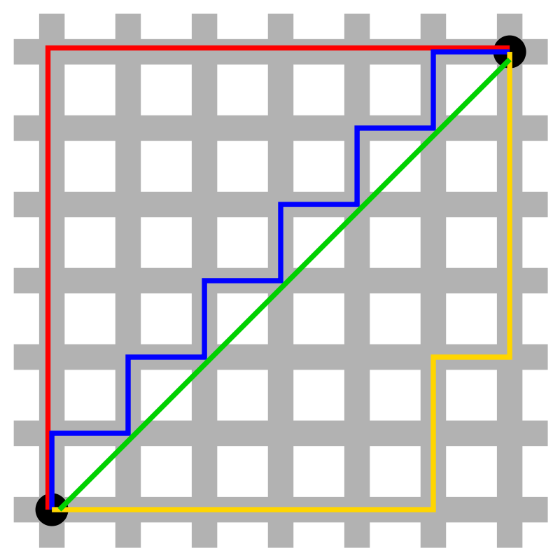

結果の表示と保存

上の関数を実行した場合、結果が保存される dis.bc は dist というクラスの下三角行列 になる。

行と列の名前は、1 - 20 の site になり、つまり 1 と 2 の群集がどれくらい似ているか、1 と 3, 1 と 4 ... 19 と 20 という総当たりの比較がデータとして出てくるわけである。

ただし、これを書き出すにはちょっと工夫が必要。

普通に以下のように書き出しを実行すると、Error in as.data.frame.default (x[[i]], optional = TRUE) : cannot coerce class ‘"dist"’ to a data.frame というエラーになる。形を見てわかるとおり、確かにデータフレームとは少し違っている。

write.csv(dis.bc, file = "a.csv")

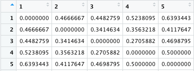
この dist というクラスはかなり扱いづらいので、csv などに書き出したいのなら、最初から as.matrix としておく (3)。

dis.bc2 <- as.matrix(vegdist(dune, method = "bray"))

こうすると dis.bc2 は対角線に 0 がある対称行列となる。1 - 5 のみを示しておくが、20 x 20 である。これは write.csv などで書き出すことができる。

cmdscale() および ggplot() による図の作成

以上のようにして計算された β 多様性 dis.bc2 は、距離行列である。これは、しばしば二次元平面上にプロットして視覚化される。

このように、高次元のデータを 2 - 3 次元に落として視覚化するための分析手法を 主座標分析 (principal coordinate analysis, PCoA) という。したがって、以下の内容は 主座標分析 PCoA のページ の内容と一部重複する。詳しく知りたい人は、リンク先も参照のこと。

cmdscale() は、classical multidimensional scaling を行う関数である。これは主座標分析と同じであると RDocumentation に書かれている。

このページの上の方で行ったように、dune データセットの bray 距離を計算し、それを matrix にする。さらに、その matrix を cmdscale で処理すると、総当たりだった距離が V1 と V2 という 2 つの変数にまとめられる。

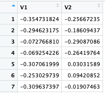
こうなれば、V1 と V2 を散布図にしてやればよい。ggplot はデータフレームを input にするので、as.data.frame をつけるのを忘れないこと。

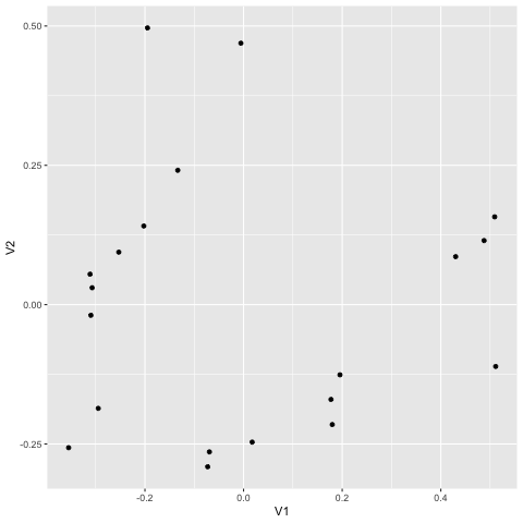
図には 20 個の点があり、dune の 1 - 20 番に相当する。似ているデータは近くに、似ていないデータは遠くに配置されている。番号が見えないので不完全なプロットであるが (時間があるときに更新)、どのサンプルが似ているかが一目瞭然にわかることになる。

文献からの例 (4)。ただし、marked separation と書いてあるものの、NW と OB はそんなに離れていない気がする。

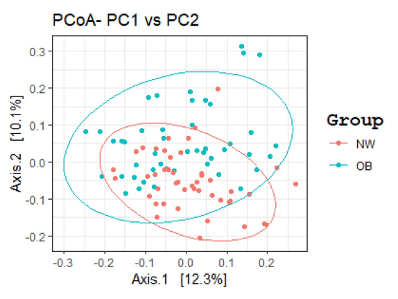
Figure 1. GM beta diversity analysis of OB patients compared to NW. Principal Coordinates Analysis (PCoA) based on Bray–Curtis distance matrix, performed in R software v.3.5.2 (ggplot2 package), showed a marked separation between the GM communities of OB and NW. The statistical significance among the two groups was determined with Permutational Multivariate Analysis of Variance (PERMANOVA) (R-vegan, function adonis), adjusted for sex, age and smoking status (sum of squares = 0.5492, mean of squares = 5.0297, F = 0.0533, R = 0.047, p = 0.002). p equal to or less than 0.05 was considered statistically significant.

文献 5。Unweighted UniFrac, Weighted UniFrac, Jaccard, Bray-Curtis を全部プロットしている。

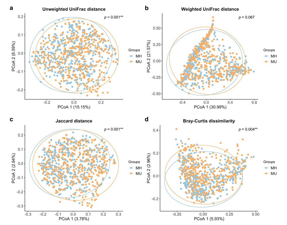
Figure 2. Principal Coordinate Analysis (PCoA) plots of beta diversity. Statistical significance between metabolically healthy (MH) and metabolically unhealthy (MU) groups using distance matrices for beta- diversity: (a) unweighted UniFrac distance, (b) weighted UniFrac distance, (c) Jaccard distance, and (d) Bray– Curtis dissimilarity indices. Statistics were calculated using pairwise PERMANOVA with 999 permutations. **p < 0.01. Ellipses represent 95% confidence interval for each group.

References

1. 多様性指数の算出：R備忘録. Link: Last access 2022/05/03.
2. Vegan turotial. Link: Last access 2022/05/03.
3. Rによるクラスター分析【ユークリッド距離】Link: Last access 2022/03/21.
4. Palmas et al., 2021a. Gut microbiota markers associated with obesity and overweight in Italian adults. Sci Rep 11, 5532.
5. Kim et al., 2020a. Gut microbiota and metabolic health among overweight and obese individuals. Sci Rep 10, 19417.

コメント欄

サーバー移転のため、コメント欄は一時閉鎖中です。サイドバーから「管理人への質問」へどうぞ。

↑